m <- matrix(1:25, nrow = 5, ncol = 5)
m
# [,1] [,2] [,3] [,4] [,5]
# [1,] 1 6 11 16 21
# [2,] 2 7 12 17 22
# [3,] 3 8 13 18 23
# [4,] 4 9 14 19 24
# [5,] 5 10 15 20 25
grid_data_test <- expand.grid(row = 1:5, col = 1:5)
grid_data_test
# row col
# 1 1 1
# 2 2 1
# 3 3 1
# 4 4 1
# 5 5 1
# 6 1 2
# 7 2 2
# 8 3 2
# 9 4 2
# 10 5 2
# 11 1 3
# 12 2 3
# 13 3 3
# 14 4 3
# 15 5 3
# 16 1 4
# 17 2 4
# 18 3 4
# 19 4 4
# 20 5 4
# 21 1 5
# 22 2 5
# 23 3 5
# 24 4 5
# 25 5 5
grid_data_test$probs <- reshape2::melt(m)[, 3]
grid_data_test
# row col probs
# 1 1 1 1
# 2 2 1 2
# 3 3 1 3
# 4 4 1 4
# 5 5 1 5
# 6 1 2 6
# 7 2 2 7
# 8 3 2 8
# 9 4 2 9
# 10 5 2 10
# 11 1 3 11
# 12 2 3 12
# 13 3 3 13
# 14 4 3 14
# 15 5 3 15
# 16 1 4 16
# 17 2 4 17
# 18 3 4 18
# 19 4 4 19
# 20 5 4 20
# 21 1 5 21
# 22 2 5 22
# 23 3 5 23
# 24 4 5 24
# 25 5 5 25
# Plot
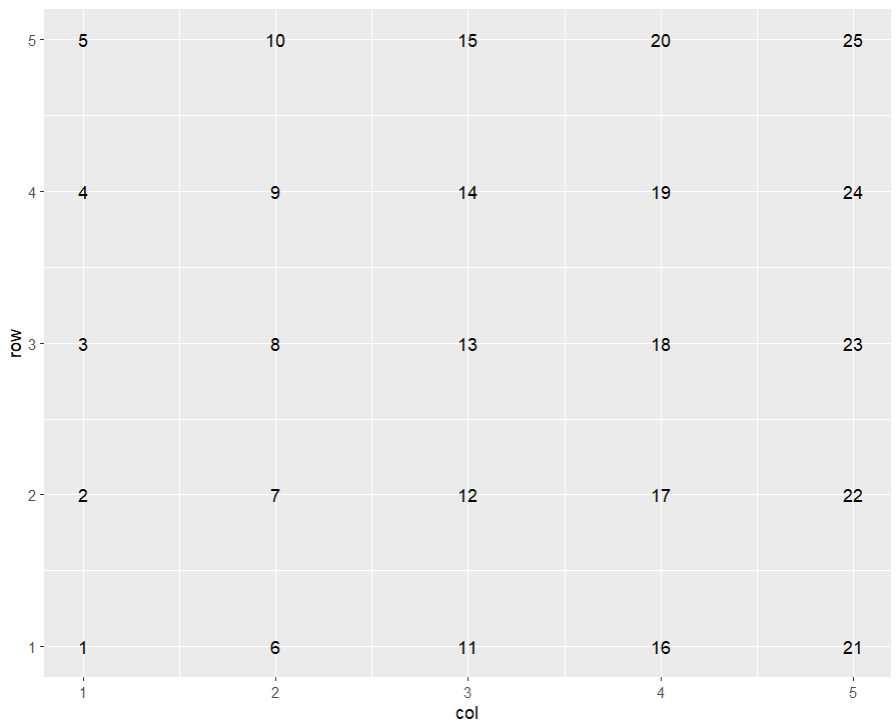
ggplot(grid_data_test, aes(x = col, y = row, label = round(probs, 2))) +
geom_text()The Ellsworth Project: Part 4
R
Shiny
Documenting the creation of The Ellsworth App, in which I figure out why my probability mapping is wonky in my plots.
February 24th, 2024
Very little chance to code today, but now that I know what’s up, maybe I can make some quick changes and go to bed happy? I’m creating a matrix correctly, everything looks right before and after I melt it. Why is ggplot reversing the order that my columns are plotting? It’s getting everything else right, just reversing the order of each column. And I commented out the geom_tile call yesterday, so it’s not geom_tile itself. How else can I test this? I need to plot without the theming.
[Note from Future Libby: Y’all, she is gonna feel so silly in a minute, just watch.]
OMG DUHHHHH, of course the axes go from 0 in the bottom left corner! It’s not reversing it, I’m the one NOT reversing the axes! That’s why the columns are in order and the rows are just backwards. Ok, SHEW. Yeah, don’t code tired, Libby. That was dumb 😂 Let me do this again, without the Tired Libby mistakes.
ggplot(grid_data_test, aes(x = col, y = row, label = round(probs, 2))) +
    geom_text() +
        scale_y_reverse() +
        coord_fixed()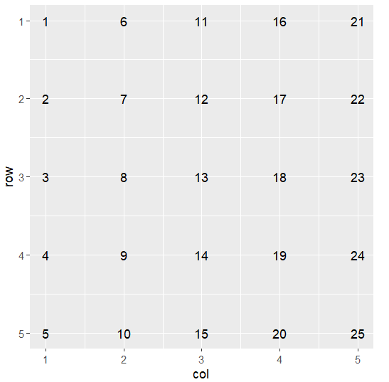
YAAAAAAAAS.
# Load packages
library(tidyverse)

# Define a function to generate a random vector of colors
generate_color_vector <- function(size, colors) {

  # Create a size^2 vector filled with a random sample of colors from a color list
  color_vector <- sample(x = colors,
                         size = size * size,   # "size" is the # of squares on each side
                         replace = TRUE)

  return(color_vector)
}

# Set the size of the desired grid and calculate number of circuits
size <- 40
circuits <- ifelse(size %% 2 == 0, size/2, (size+1)/2)

# Define the colors
colors <- c(#"#EDEFEE", # Paper
            "#1A8BB3", # Teal - no longer teal, just bright blue
            "#0950AE", # Dark blue
            "#4DACE5", # Light blue
            "#126DDB", # Blue
            "#E48DC4", # Pink
            "#ABA9E8", # Light purple
            "#872791", # Purple
            "#6D1617", # Dark red
            "#B81634", # Red
            "#DF3B43", # Red orange
            "#E35C47", # Orange
            "#EB8749", # Light orange
            "#F6E254", # Yellow
            "#7B442D", # Brown
            "#000000", # Black
            "#1A6E7E", # Dark green - no longer dark green, now looks teal
            "#7CBF7B", # Green
            "#ADD2B8") # Light green

# Generate the color grid
color_vector <- generate_color_vector(size, colors)

# Create a data frame for the grid coordinates
df <- expand.grid(x = 1:size, y = 1:size)

# Add the corresponding color to each grid cell coordinate
df$color <- color_vector

# Include my function that calculates probabilities based on circuits
# Maybe I should make it based on size? I will already have circuits, though.
get_prob_vector <- function(circuits){

  first10perc <- seq(0, 0.02857143, length.out = round(circuits*.10)+1) # 3

  last90perc_length <- circuits - length(first10perc)

  last10perc_length <- round(last90perc_length * (1/9)) # 2

  middle80perc_length <- last90perc_length - last10perc_length # 15

  middle80perc <- seq(0.02857143, 1, length.out = middle80perc_length+2)[-c(1, middle80perc_length+2)]

  last10perc <- rep(1, last10perc_length)

  prob_vector <- c(first10perc, middle80perc, last10perc)

  return(prob_vector)
}

prob_vector <- get_prob_vector(circuits)

# Create function that builds the prob matrix
get_prob_matrix <- function(size, prob_vector){

  # Calculate quad size same way as circuits
  quad_size <- ifelse(size %% 2 == 0, size/2, (size+1)/2)

  # Create empty matrix for the quad
  M <- matrix(0, nrow = quad_size, ncol = quad_size)

  # For loop to assign prob_vector to correct cells in quadrant
  for (i in 1:quad_size){

    M[i, i:quad_size] <- prob_vector[i]
    M[i:quad_size, i] <- prob_vector[i]
  }

  # if size is even,
  if(size %% 2 == 0){
    # mirror horizontally and column bind
    M_right <- apply(M, 1, rev)
    M <- cbind(M, M_right)

    # then mirror vertically and row bind
    M_down <- apply(M, 2, rev)
    M <- rbind(M, M_down)

  }else{ # if size is odd
    # mirror all but last col horizontally and col bind
    M_right <- apply(M[ , 1:(quad_size-1)], 1, rev)
    M <- cbind(M, M_right)

    # then mirror all but last row vertically and row bind
    M_down <- apply(M[1:(quad_size-1), ], 2, rev)
    M <- rbind(M, M_down)

  }

  return(M)
}

M <- get_prob_matrix(size, prob_vector)


# Apply M to df as a vector
df$probs <- as.vector(M)

# Plot, but make sure the y axis is reversed

ggplot(df, aes(x = x, y = y, label = round(probs, 2))) +
  geom_tile(aes(fill = probs), colour = "white") +
    geom_text() +
        scale_y_reverse() +
    scale_fill_gradient(low = "white", high = "blue") +
    theme_minimal() +
    theme(axis.text = element_blank(),
          axis.title = element_blank(),
          panel.grid = element_blank(),
          plot.margin = margin(1, 1, 1, 1, "cm")) +
    coord_fixed()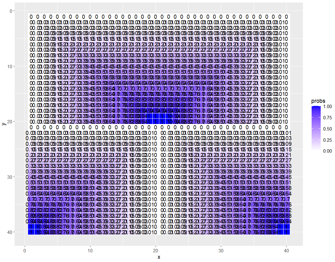
That’s progress, baybeeeee! Now that I know my axes are going in the right directions, I can focus on where I think the actual problem is happening, which is in the flipping and binding of the matrices. I’m going to make a minimum viable example to test that function and see what’s going on at each step.
This is the guts of the function that takes the quadrant M and flips it horizontally, then cbinds it, then flips that vertically and rbinds that. Maybe I’m getting the arguments wrong and mixing things up. Lemme see what each thing is doing.
# smol zample
size <- 12
circuits <- ifelse(size %% 2 == 0, size/2, (size+1)/2)

# This is a test, so I'm gonna use a smaller prob_vector, too
prob_vector <- get_prob_vector(circuits)

# Calculate quad size same way as circuits
quad_size <- ifelse(size %% 2 == 0, size/2, (size+1)/2)

# Create empty matrix for the quad
M <- matrix(0, nrow = quad_size, ncol = quad_size)

M
#      [,1] [,2] [,3] [,4] [,5] [,6]
# [1,]    0    0    0    0    0    0
# [2,]    0    0    0    0    0    0
# [3,]    0    0    0    0    0    0
# [4,]    0    0    0    0    0    0
# [5,]    0    0    0    0    0    0
# [6,]    0    0    0    0    0    0

# For loop to assign prob_vector to correct cells in quadrant
for (i in 1:quad_size){

  M[i, i:quad_size] <- prob_vector[i]
  M[i:quad_size, i] <- prob_vector[i]
}

round(M, 2)
#      [,1] [,2] [,3] [,4] [,5] [,6]
# [1,]    0 0.00 0.00 0.00 0.00 0.00
# [2,]    0 0.03 0.03 0.03 0.03 0.03
# [3,]    0 0.03 0.22 0.22 0.22 0.22
# [4,]    0 0.03 0.22 0.42 0.42 0.42
# [5,]    0 0.03 0.22 0.42 0.61 0.61
# [6,]    0 0.03 0.22 0.42 0.61 0.81

# ^ Wow, good to know my prob_vector is failing at this small size. Should have known.
# I can add a condition for that later.

# mirror horizontally and column bind
  M_right <- apply(M, 1, rev)

round(M_right, 2)
#      [,1] [,2] [,3] [,4] [,5] [,6]
# [1,]    0 0.03 0.22 0.42 0.61 0.81
# [2,]    0 0.03 0.22 0.42 0.61 0.61
# [3,]    0 0.03 0.22 0.42 0.42 0.42
# [4,]    0 0.03 0.22 0.22 0.22 0.22
# [5,]    0 0.03 0.03 0.03 0.03 0.03
# [6,]    0 0.00 0.00 0.00 0.00 0.00

# ah hah! It's mirroring it up-down, not left-right.
# in apply(), 1 indicates rows, 2 indicates columns, so I just got the argument wrong.
# I need to reverse the columns, not the rows, in order to mirror it horizontally

# Try that again with the right arg
M_right <- apply(M, 2, rev)

round(M_right, 2)
#      [,1] [,2] [,3] [,4] [,5] [,6]
# [1,]    0 0.03 0.22 0.42 0.61 0.81
# [2,]    0 0.03 0.22 0.42 0.61 0.61
# [3,]    0 0.03 0.22 0.42 0.42 0.42
# [4,]    0 0.03 0.22 0.22 0.22 0.22
# [5,]    0 0.03 0.03 0.03 0.03 0.03
# [6,]    0 0.00 0.00 0.00 0.00 0.00

# Ok, wait. What? The result of apply(M, 2, rev) and apply(M, 1, rev) are the same?
test1 <- round(apply(M, 1, rev), 2)
test2 <- round(apply(M, 2, rev), 2)

identical(test1, test2)
# [1] TRUE

# Great. That means I have just been wasting time with rev :D Should have used pracma!
Womp womp. Why didn’t I use pracma or raster to begin with? I wasn’t mirroring in the way I thought I was 😂 I’m gonna test pracma::flipud and fliplr (which I think stand for flip up down and flip left right).
library(pracma)

# smol zample, but larger than 12, let's test 16
size <- 16
circuits <- ifelse(size %% 2 == 0, size/2, (size+1)/2)

# This is a test, so I'm gonna use a smaller prob_vector, too
prob_vector <- get_prob_vector(circuits)

# Calculate quad size same way as circuits
quad_size <- ifelse(size %% 2 == 0, size/2, (size+1)/2)

# Create empty matrix for the quad
M <- matrix(0, nrow = quad_size, ncol = quad_size)
M
#      [,1] [,2] [,3] [,4] [,5] [,6] [,7] [,8]
# [1,]    0    0    0    0    0    0    0    0
# [2,]    0    0    0    0    0    0    0    0
# [3,]    0    0    0    0    0    0    0    0
# [4,]    0    0    0    0    0    0    0    0
# [5,]    0    0    0    0    0    0    0    0
# [6,]    0    0    0    0    0    0    0    0
# [7,]    0    0    0    0    0    0    0    0
# [8,]    0    0    0    0    0    0    0    0

# For loop to assign prob_vector to correct cells in quadrant
for (i in 1:quad_size){

  M[i, i:quad_size] <- prob_vector[i]
  M[i:quad_size, i] <- prob_vector[i]
}

round(M, 2)
#      [,1] [,2] [,3] [,4] [,5] [,6] [,7] [,8]
# [1,]    0 0.00 0.00 0.00 0.00 0.00 0.00 0.00
# [2,]    0 0.03 0.03 0.03 0.03 0.03 0.03 0.03
# [3,]    0 0.03 0.19 0.19 0.19 0.19 0.19 0.19
# [4,]    0 0.03 0.19 0.35 0.35 0.35 0.35 0.35
# [5,]    0 0.03 0.19 0.35 0.51 0.51 0.51 0.51
# [6,]    0 0.03 0.19 0.35 0.51 0.68 0.68 0.68
# [7,]    0 0.03 0.19 0.35 0.51 0.68 0.84 0.84
# [8,]    0 0.03 0.19 0.35 0.51 0.68 0.84 1.00

# ^ prob vector function is mostly ok at this size, but this may be as small as
# I can go. Maybe I can create a series of plots to test visually once I'm done,
# then use the results for my conditionals on size instead of limiting
# the function itself.

# mirror horizontally and column bind
M_right <- pracma::fliplr(M)

round(M_right, 2)
#      [,1] [,2] [,3] [,4] [,5] [,6] [,7] [,8]
# [1,] 0.00 0.00 0.00 0.00 0.00 0.00 0.00    0
# [2,] 0.03 0.03 0.03 0.03 0.03 0.03 0.03    0
# [3,] 0.19 0.19 0.19 0.19 0.19 0.19 0.03    0
# [4,] 0.35 0.35 0.35 0.35 0.35 0.19 0.03    0
# [5,] 0.51 0.51 0.51 0.51 0.35 0.19 0.03    0
# [6,] 0.68 0.68 0.68 0.51 0.35 0.19 0.03    0
# [7,] 0.84 0.84 0.68 0.51 0.35 0.19 0.03    0
# [8,] 1.00 0.84 0.68 0.51 0.35 0.19 0.03    0
That looks… right O_O omgomgomg. Lemme test the flipud() part. Gotta finish binding that first set of matrices, though.
M <- cbind(M, M_right)

round(M, 2)
#      [,1] [,2] [,3] [,4] [,5] [,6] [,7] [,8] [,9] [,10] [,11] [,12] [,13] [,14] [,15] [,16]
# [1,]    0 0.00 0.00 0.00 0.00 0.00 0.00 0.00 0.00  0.00  0.00  0.00  0.00  0.00  0.00     0
# [2,]    0 0.03 0.03 0.03 0.03 0.03 0.03 0.03 0.03  0.03  0.03  0.03  0.03  0.03  0.03     0
# [3,]    0 0.03 0.19 0.19 0.19 0.19 0.19 0.19 0.19  0.19  0.19  0.19  0.19  0.19  0.03     0
# [4,]    0 0.03 0.19 0.35 0.35 0.35 0.35 0.35 0.35  0.35  0.35  0.35  0.35  0.19  0.03     0
# [5,]    0 0.03 0.19 0.35 0.51 0.51 0.51 0.51 0.51  0.51  0.51  0.51  0.35  0.19  0.03     0
# [6,]    0 0.03 0.19 0.35 0.51 0.68 0.68 0.68 0.68  0.68  0.68  0.51  0.35  0.19  0.03     0
# [7,]    0 0.03 0.19 0.35 0.51 0.68 0.84 0.84 0.84  0.84  0.68  0.51  0.35  0.19  0.03     0
# [8,]    0 0.03 0.19 0.35 0.51 0.68 0.84 1.00 1.00  0.84  0.68  0.51  0.35  0.19  0.03     0

# Looks promising!

M_down <- pracma::flipud(M)

round(M_down, 2)
#      [,1] [,2] [,3] [,4] [,5] [,6] [,7] [,8] [,9] [,10] [,11] [,12] [,13] [,14] [,15] [,16]
# [1,]    0 0.03 0.19 0.35 0.51 0.68 0.84 1.00 1.00  0.84  0.68  0.51  0.35  0.19  0.03     0
# [2,]    0 0.03 0.19 0.35 0.51 0.68 0.84 0.84 0.84  0.84  0.68  0.51  0.35  0.19  0.03     0
# [3,]    0 0.03 0.19 0.35 0.51 0.68 0.68 0.68 0.68  0.68  0.68  0.51  0.35  0.19  0.03     0
# [4,]    0 0.03 0.19 0.35 0.51 0.51 0.51 0.51 0.51  0.51  0.51  0.51  0.35  0.19  0.03     0
# [5,]    0 0.03 0.19 0.35 0.35 0.35 0.35 0.35 0.35  0.35  0.35  0.35  0.35  0.19  0.03     0
# [6,]    0 0.03 0.19 0.19 0.19 0.19 0.19 0.19 0.19  0.19  0.19  0.19  0.19  0.19  0.03     0
# [7,]    0 0.03 0.03 0.03 0.03 0.03 0.03 0.03 0.03  0.03  0.03  0.03  0.03  0.03  0.03     0
# [8,]    0 0.00 0.00 0.00 0.00 0.00 0.00 0.00 0.00  0.00  0.00  0.00  0.00  0.00  0.00     0

M <- rbind(M, M_down)

grid_data_smol <- expand.grid(row = 1:16, col = 1:16)
grid_data_smol$probs <- as.vector(M) # why did I leave you, as.vector? #base4lyfe

ggplot(grid_data_smol, aes(x = col, y = row, label = round(probs, 2))) +
  geom_tile(aes(fill = probs), colour = "white") +
  geom_text() +
  scale_fill_gradient(low = "white", high = "blue") +
  theme_minimal() +
  theme(axis.text = element_blank(),
        axis.title = element_blank(),
        panel.grid = element_blank(),
        plot.margin = margin(1, 1, 1, 1, "cm")) +
  coord_fixed()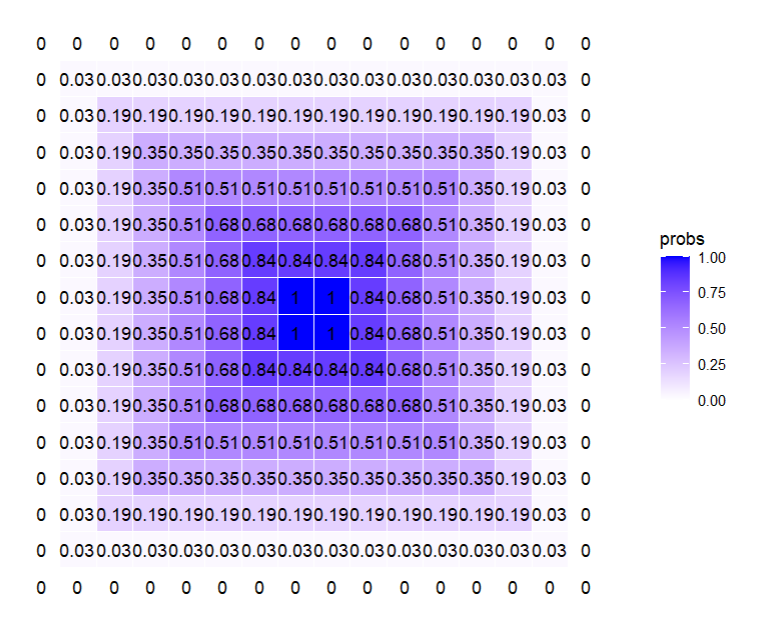
😭 I AM SO HAPPY! AGAIN!
# Load packages
library(tidyverse)
library(pracma)

# Define a function to generate a random vector of colors
generate_color_vector <- function(size, colors) {

  # Create a size^2 vector filled with a random sample of colors from a color list
  color_vector <- sample(x = colors,
                         size = size * size,   # "size" is the # of squares on each side
                         replace = TRUE)

  return(color_vector)
}

# Set the size of the desired grid and calculate number of circuits
size <- 40
circuits <- ifelse(size %% 2 == 0, size/2, (size+1)/2)

# Define the colors
colors <- c(#"#EDEFEE", # Paper
            "#1A8BB3", # Teal - no longer teal, just bright blue
            "#0950AE", # Dark blue
            "#4DACE5", # Light blue
            "#126DDB", # Blue
            "#E48DC4", # Pink
            "#ABA9E8", # Light purple
            "#872791", # Purple
            "#6D1617", # Dark red
            "#B81634", # Red
            "#DF3B43", # Red orange
            "#E35C47", # Orange
            "#EB8749", # Light orange
            "#F6E254", # Yellow
            "#7B442D", # Brown
            "#000000", # Black
            "#1A6E7E", # Dark green - no longer dark green, now looks teal
            "#7CBF7B", # Green
            "#ADD2B8") # Light green

# Generate the color grid
color_vector <- generate_color_vector(size, colors)

# Create a data frame for the grid coordinates
df <- expand.grid(x = 1:size, y = 1:size)

# Add the corresponding color to each grid cell coordinate
df$color <- color_vector

# Include my function that calculates probabilities based on circuits
# Maybe I should make it based on size? I will already have circuits, though.
get_prob_vector <- function(circuits){

  first10perc <- seq(0, 0.02857143, length.out = round(circuits*.10)+1) # 3

  last90perc_length <- circuits - length(first10perc)

  last10perc_length <- round(last90perc_length * (1/9)) # 2

  middle80perc_length <- last90perc_length - last10perc_length # 15

  middle80perc <- seq(0.02857143, 1, length.out = middle80perc_length+2)[-c(1, middle80perc_length+2)]

  last10perc <- rep(1, last10perc_length)

  prob_vector <- c(first10perc, middle80perc, last10perc)

  return(prob_vector)
}

prob_vector <- get_prob_vector(circuits)

# Create function that builds the prob matrix
get_prob_matrix <- function(size, prob_vector){

  # Calculate quad size same way as circuits
  quad_size <- ifelse(size %% 2 == 0, size/2, (size+1)/2)

  # Create empty matrix for the quad
  M <- matrix(0, nrow = quad_size, ncol = quad_size)

  # For loop to assign prob_vector to correct cells in quadrant
  for (i in 1:quad_size){

    M[i, i:quad_size] <- prob_vector[i]
    M[i:quad_size, i] <- prob_vector[i]
  }

  # if quad_size is even,
  if(quad_size %% 2 == 0){
    # mirror horizontally and column bind
    M_right <- pracma::fliplr(M)
    M <- cbind(M, M_right)

    # then mirror vertically and row bind
    M_down <- pracma::flipud(M)
    M <- rbind(M, M_down)

  }else{ # if quad_size is odd
    # mirror all but last col horizontally and col bind
    M_right <- pracma::fliplr(M[ , 1:(quad_size-1)])
    M <- cbind(M, M_right)

    # then mirror all but last row vertically and row bind
    M_down <- pracma::flipud(M[1:(quad_size-1), ])
    M <- rbind(M, M_down)

  }

  return(M)
}

M <- get_prob_matrix(size, prob_vector)


# Apply M to df as a vector
df$probs <- as.vector(M)

# Plot, but make sure the y axis is reversed

ggplot(df, aes(x = x, y = y, label = round(probs, 2))) +
  geom_tile(aes(fill = probs), colour = "white") +
    geom_text() +
    scale_fill_gradient(low = "white", high = "blue") +
        scale_y_reverse() +
    theme_minimal() +
    theme(axis.text = element_blank(),
          axis.title = element_blank(),
          panel.grid = element_blank(),
          plot.margin = margin(1, 1, 1, 1, "cm")) +
    coord_fixed()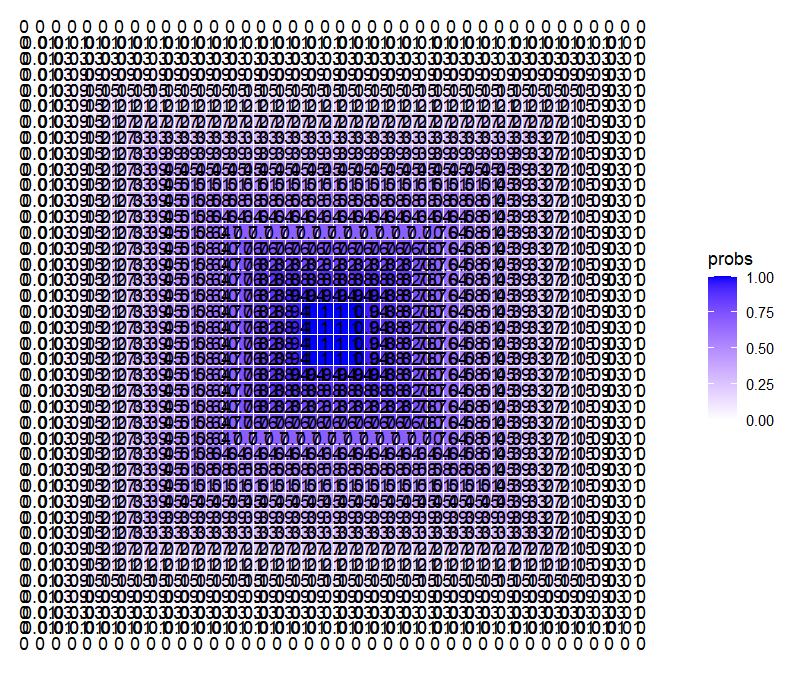
Can you even handle it?!? Does it work on an odd-sized grid, too? Gonna test at size 25, which will be an odd-sized grid overall, and will also have an odd-sized quad of 13.
# Set the size of the desired grid and calculate number of circuits
size <- 25
circuits <- ifelse(size %% 2 == 0, size/2, (size+1)/2)

# Generate the color grid
color_vector <- generate_color_vector(size, colors)

# Create a data frame for the grid coordinates
df <- expand.grid(x = 1:size, y = 1:size)

# Add the corresponding color to each grid cell coordinate
df$color <- color_vector

# Get the prob vector
prob_vector <- get_prob_vector(circuits)

# Get the prob matrix
M <- get_prob_matrix(size, prob_vector)

# Apply M to df as a vector
df$probs <- as.vector(M)

# Plot, but make sure the y axis is reversed

ggplot(df, aes(x = x, y = y, label = round(probs, 2))) +
  geom_tile(aes(fill = probs), colour = "white") +
    geom_text() +
    scale_fill_gradient(low = "white", high = "blue") +
        scale_y_reverse() +
    theme_void() +
    coord_fixed()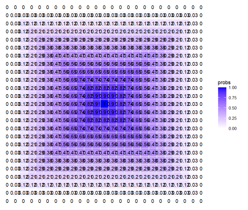
Ok 😌 Now I can go to bed happy. And before midnight! 😴 Next up is trying to map these probabilities to random samples of colors, and my initial idea for that is to recreate the Piece VII random grid and then use a sample function and a random function to assign background-color squares in the negative space using 1-prob. The random number is to compare to the prob. If it’s below (or above, whatever I want), then it will assign a white square. If not, it will do nothing. I guess using case_when(). Or something. I’ll write it out tomorrow. BED!
[Note from Future Libby: Gosh, I love her. Look at that wonder and enthusiasm. This is the best.]
I don’t know why you’re still reading this, but if you are, I’ll link the fifth post in the series here, and here’s the app in its current form if you’d like to play with it!.