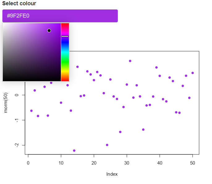
library(shiny)

shinyApp(
  ui = fluidPage(
    colourpicker::colourInput("col", "Select colour", "purple"),
    plotOutput("plot")
  ),
  server = function(input, output) {
    output$plot <- renderPlot({
      set.seed(1)
      plot(rnorm(50), bg = input$col, col = input$col, pch = 21)
    })
  }
)The Ellsworth Project: Part 5
R
Shiny
Documenting the creation of The Ellsworth App, in which I bathe in color and finally get a solid Piece III plot!
February 25th, 2024
Super tired today, so instead of working on brain-heavy stuff, I’m going to gather resources for the project. I’ll leave finishing the “piece III” prototype for tomorrow. I know I need to gather some methods of adding the functionality I want to the app, so I’ll start with a list:
- color picker for shiny app - need way to choose multiple colors
{colourpicker}
Example page: https://daattali.com/shiny/colourInput/
Example page code: https://github.com/daattali/colourpicker/blob/master/inst/examples/colourInput/app.R
- Multiple color pickers in a split issue: https://stackoverflow.com/questions/49011078/multiple-colourpickers-within-splitlayout-colour-box-gets-hidden
- Way to create a swatch or palette table/plot to show user what their color selections look like together and to also be able to save as a file along with the plot
- considered putting it in a legend at the bottom, but I’d rather it be standalone
{scales}hasshow_col():
library(scales)

# Define the colors
colors <- c(#"#EDEFEE", # Paper
  "#1A8BB3", # Teal - no longer teal, just bright blue
  "#0950AE", # Dark blue
  "#4DACE5", # Light blue
  "#126DDB", # Blue
  "#E48DC4", # Pink
  "#ABA9E8", # Light purple
  "#872791", # Purple
  "#6D1617", # Dark red
  "#B81634", # Red
  "#DF3B43", # Red orange
  "#E35C47", # Orange
  "#EB8749", # Light orange
  "#F6E254", # Yellow
  "#7B442D", # Brown
  "#000000", # Black
  "#1A6E7E", # Dark green - no longer dark green, now looks teal
  "#7CBF7B", # Green
  "#ADD2B8") # Light green

scales::show_col(colors) # I don't love that it has blank squares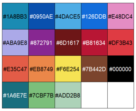
{hues}package hasswatch():
library(hues)

# Define the colors
colors <- c(#"#EDEFEE", # Paper
  "#1A8BB3", # Teal - no longer teal, just bright blue
  "#0950AE", # Dark blue
  "#4DACE5", # Light blue
  "#126DDB", # Blue
  "#E48DC4", # Pink
  "#ABA9E8", # Light purple
  "#872791", # Purple
  "#6D1617", # Dark red
  "#B81634", # Red
  "#DF3B43", # Red orange
  "#E35C47", # Orange
  "#EB8749", # Light orange
  "#F6E254", # Yellow
  "#7B442D", # Brown
  "#000000", # Black
  "#1A6E7E", # Dark green - no longer dark green, now looks teal
  "#7CBF7B", # Green
  "#ADD2B8") # Light green

hues::swatch(colors) # this is definitely more palette-like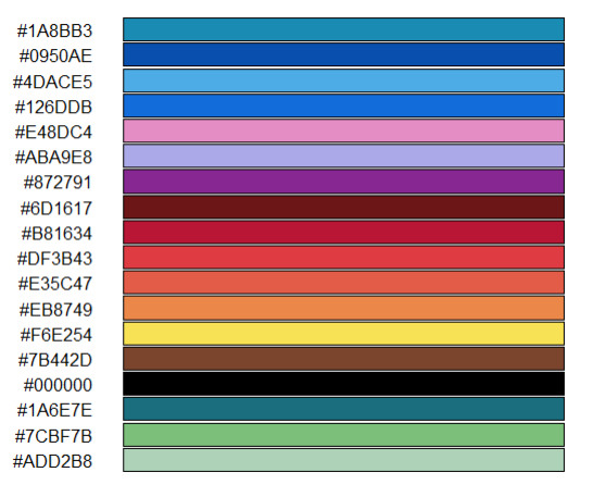
February 26th, 2024
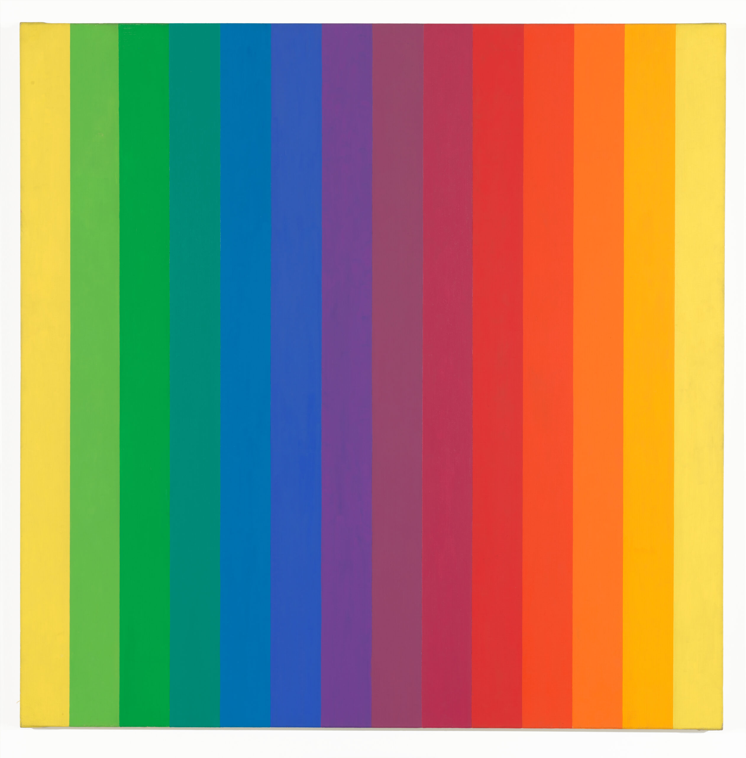
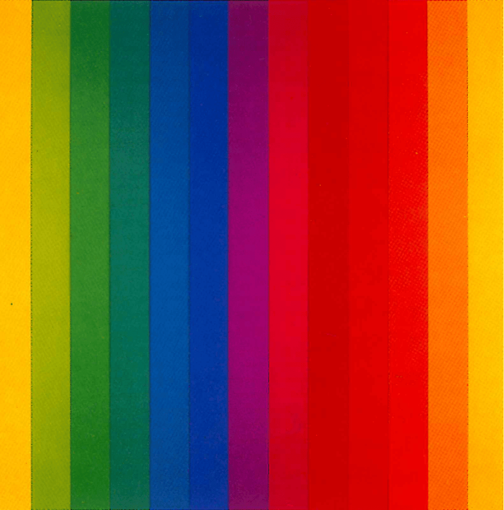
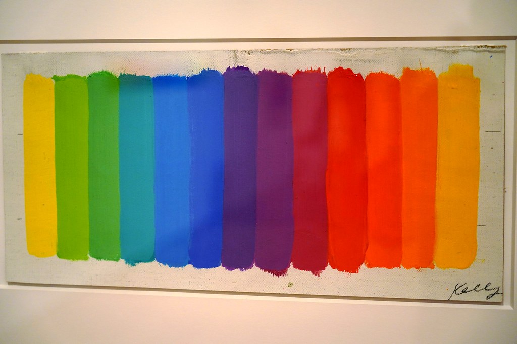
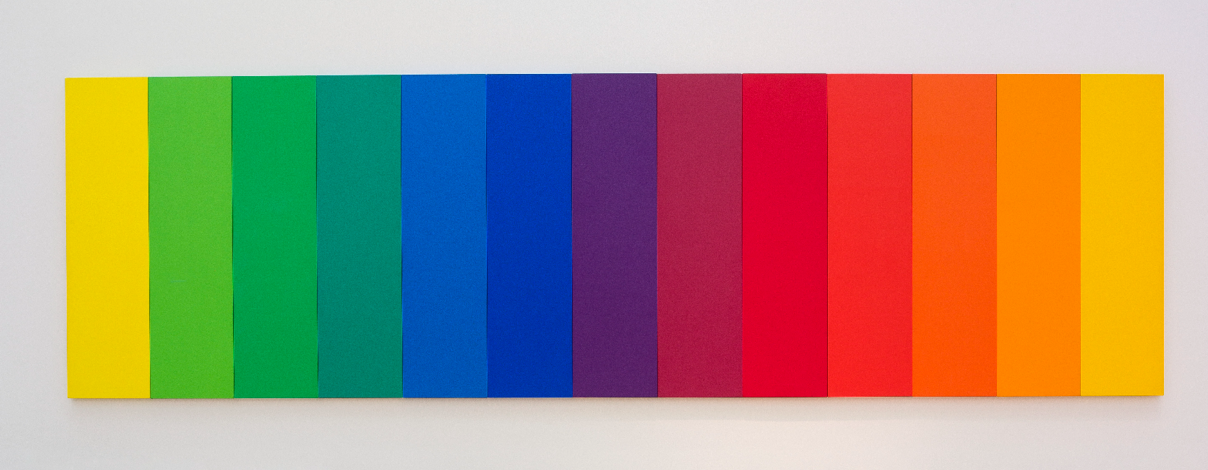
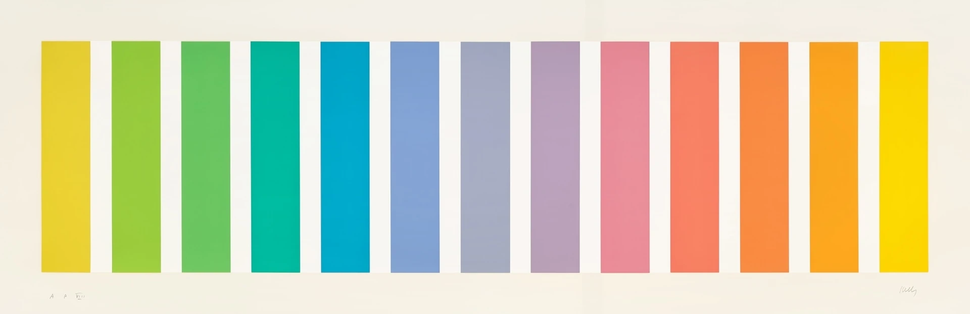
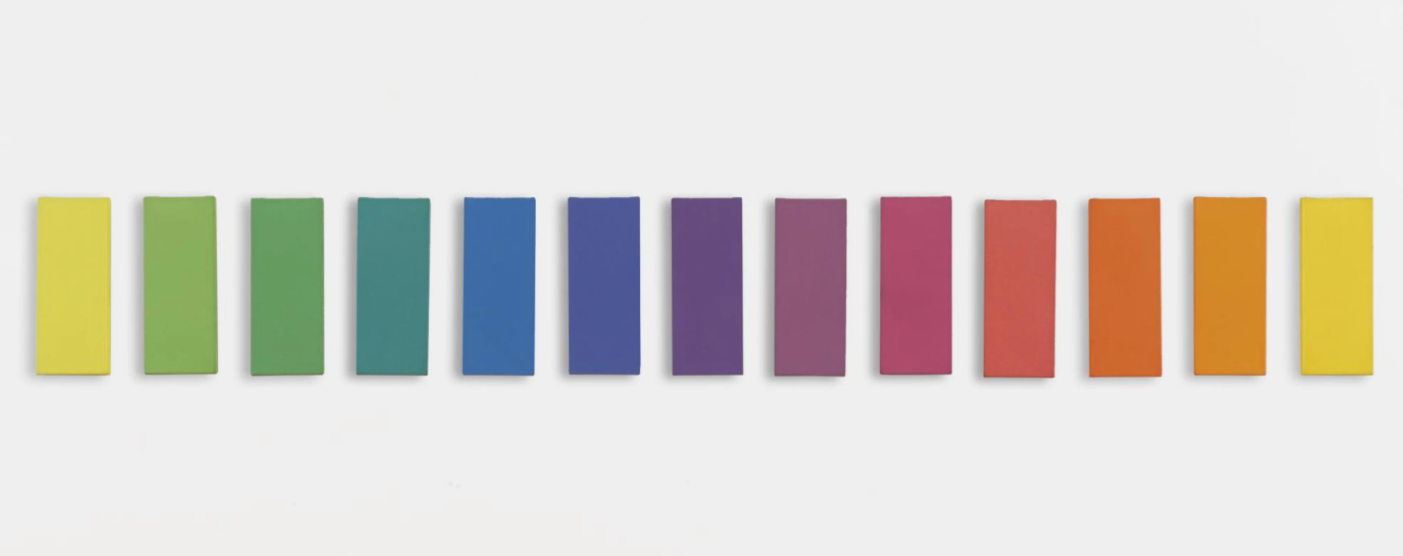
I can’t stop thinking about colors! Ellsworth is all about color, and he’s infested my brain! I want to revisit some of his other paintings and pieces for color inspiration (I say pieces because my favorite Spectrum Colors Arranged by Chance pieces are collages of paper pasted on paper, they’re not paint), because it looks like he used the same colors on other works outside of the “Arranged by Chance” series. I probably won’t re-sample or anything, I just want to bathe in the colors. The more I learn about the spectrum of visible colors, the more I realize how fascinating it is. Our ROYGBIV-style separation of colors is arbitrary - there is no dividing line between colors. It’s a continuous spectrum. The FREEDOM and ambiguity that provides is maddening and wonderful.
Ahhhh. That was a nice color bath. I needed that after having to reinstall my OS to try to revive my laptop. (Which worked! For now.) On to the final plot code! The other night, I left myself a note on what was next:
Recreate the piece VII random grid and then use a sample function and a random function to assign background-color squares in the negative space using 1-prob. The random number is to compare to the prob. If it’s below (or above, whatever I want), then it will assign a white square. If not, it will do nothing. I guess using
case_when. Or something.
That sounds pretty doable, I think. Just need to write things out. I always write things out. All my fellow aphantastics know what’s up. It all goes down on paper.
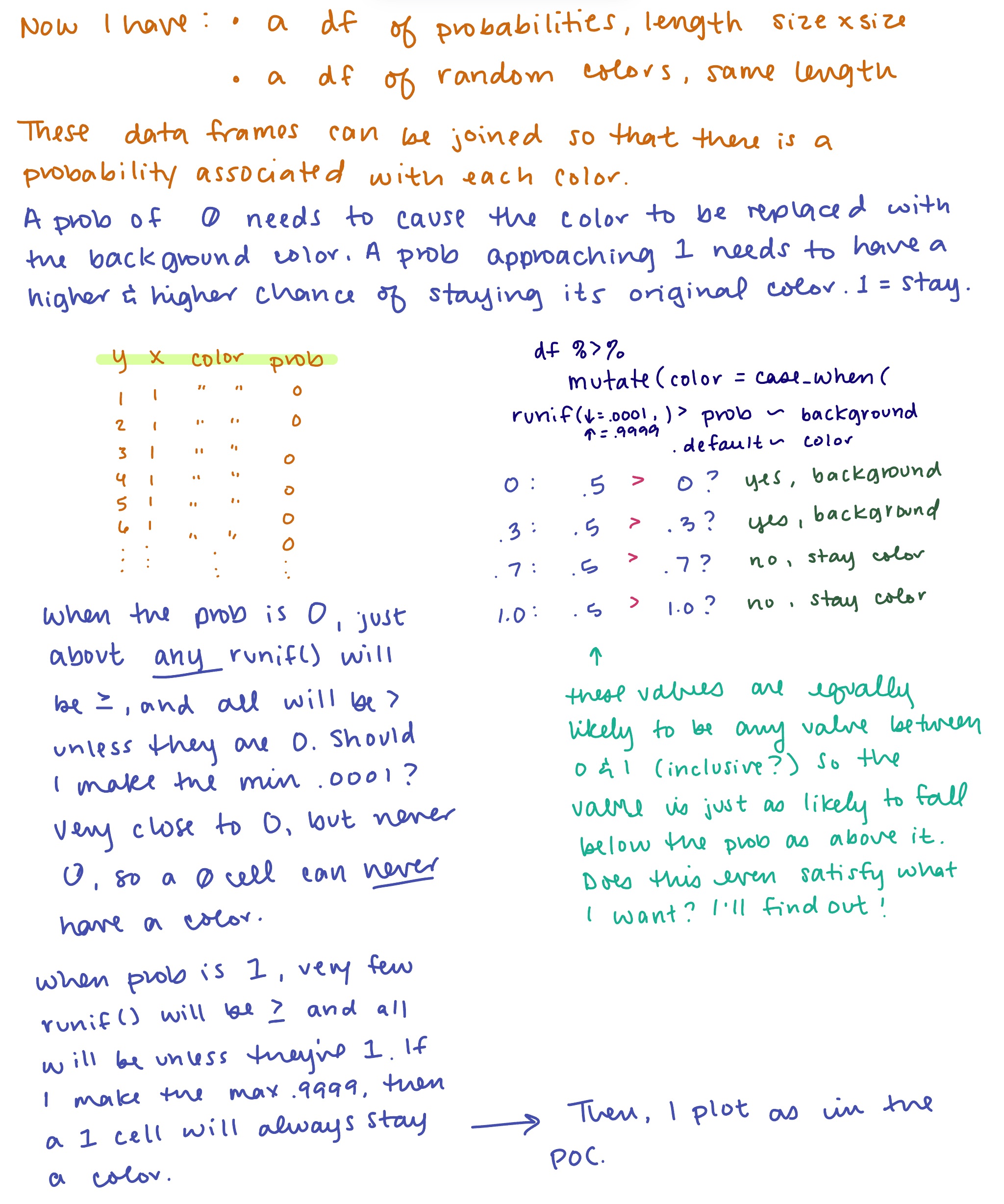
Translating those thoughts into code:
# Load packages
library(tidyverse)
library(pracma)

# Create functions needed (will source these)

# Define a function to generate a random vector of colors
generate_color_vector <- function(size, colors) {

  # Create a size^2 vector filled with a random sample of colors from a color list
  color_vector <- sample(x = colors,
                         size = size * size,   # "size" is the # of squares on each side
                         replace = TRUE)

  return(color_vector)
}

# Create function that calculates probabilities based on circuits
get_prob_vector <- function(circuits){

  first10perc <- seq(0, 0.02857143, length.out = round(circuits*.10)+1) # 3

  last90perc_length <- circuits - length(first10perc)

  last10perc_length <- round(last90perc_length * (1/9)) # 2

  middle80perc_length <- last90perc_length - last10perc_length # 15

  middle80perc <- seq(0.02857143, 1, length.out = middle80perc_length+2)[-c(1, middle80perc_length+2)]

  last10perc <- rep(1, last10perc_length)

  prob_vector <- c(first10perc, middle80perc, last10perc)

  return(prob_vector)
}

# Create function that builds the prob matrix
get_prob_matrix <- function(size, prob_vector){

  # Calculate quad size same way as circuits
  quad_size <- ifelse(size %% 2 == 0, size/2, (size+1)/2)

  # Create empty matrix for the quad
  M <- matrix(0, nrow = quad_size, ncol = quad_size)

  # For loop to assign prob_vector to correct cells in quadrant
  for (i in 1:quad_size){

    M[i, i:quad_size] <- prob_vector[i]
    M[i:quad_size, i] <- prob_vector[i]
  }

  # if size is even,
  if(size %% 2 == 0){
    # mirror horizontally and column bind
    M_right <- pracma::fliplr(M)
    M <- cbind(M, M_right)

    # then mirror vertically and row bind
    M_down <- pracma::flipud(M)
    M <- rbind(M, M_down)

  }else{ # if size is odd
    # mirror all but last col horizontally and col bind
    M_right <- pracma::fliplr(M[ , 1:(quad_size-1)])
    M <- cbind(M, M_right)

    # then mirror all but last row vertically and row bind
    M_down <- pracma::flipud(M[1:(quad_size-1), ])
    M <- rbind(M, M_down)

  }

  return(M)
}

# Set parameters (size and color will be user inputs eventually)

# Set the size of the desired grid and calculate number of circuits
size <- 40
circuits <- ifelse(size %% 2 == 0, size/2, (size+1)/2)

# Define the colors
colors <- c(#"#EDEFEE", # Paper
  "#1A8BB3", # Teal - no longer teal, just bright blue
  "#0950AE", # Dark blue
  "#4DACE5", # Light blue
  "#126DDB", # Blue
  "#E48DC4", # Pink
  "#ABA9E8", # Light purple
  "#872791", # Purple
  "#6D1617", # Dark red
  "#B81634", # Red
  "#DF3B43", # Red orange
  "#E35C47", # Orange
  "#EB8749", # Light orange
  "#F6E254", # Yellow
  "#7B442D", # Brown
  "#000000", # Black
  "#1A6E7E", # Dark green - no longer dark green, now looks teal
  "#7CBF7B", # Green
  "#ADD2B8") # Light green

# End user parameters

# Generate the color vector
color_vector <- generate_color_vector(size, colors)

# Create a data frame for the grid coordinates
df <- expand.grid(x = 1:size, y = 1:size)

# Add the corresponding color to each grid cell coordinate
df$color <- color_vector

# Get the probability vector
prob_vector <- get_prob_vector(circuits)

# Assign probabilityes to matrix correctly
M <- get_prob_matrix(size, prob_vector)

# Apply prob matrix M to df as a vector
df$probs <- as.vector(M)

#######################
# New stuff starts here:

df <-
  df |> mutate(color = case_when(
    runif(n = 1,
          min = .0001,
          max = .9999) > probs ~ background,
    .default = color
  ))

#######################
# End new stuff

# Check to see if the probs mapped correctly (yes, they did)
ggplot(df, aes(x = x, y = y, label = round(probs, 3))) +
  geom_tile(aes(fill = probs), colour = "white") +
    geom_text() +
    scale_fill_gradient(low = "white", high = "blue") +
        scale_y_reverse() +
    theme_void() +
    coord_fixed()

# Plot
kelly_colors_III <-
  ggplot(df, aes(x = x, y = y, fill = color)) +
  geom_tile() +  # Add tiles
  scale_fill_identity() +  # Use the colors stored as strings in the color column
  theme_void() +  # Remove axis labels and background
  coord_equal()  # Use equal aspect ratio

# Print the plot
kelly_colors_III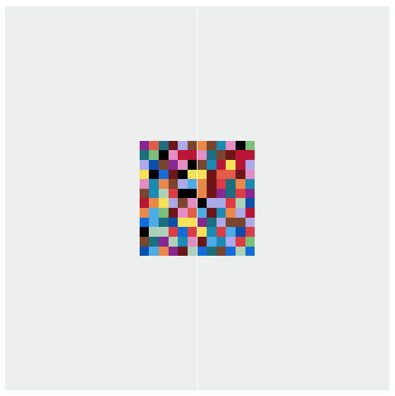
Hahaha, oh boyyyyy! Ok, well, I got what I wanted in a VERY binary sense. I just realized I only grabbed ONE runif() value 😂 Hilarious. I need to grab a fresh one for each element of the size x size vector. First of all, I’m gonna get rid of the min and max arguments and just write a condition declaring the 0 and 1 states. Then, change my case_when section so that I’m iterating over the vector element by element with a fresh runif() pull each time. This should be a function, not a mutate.
# Create a function that creates a new color column to replace the old one
get_kelly_III_vector <- function(df, background){
# Write a loop that iterates over each row in df
for (i in 1:nrow(df)){
if (df$probs[i] == 0){
df$color[i] <- background
} else if (df$probs[i] == 1){
df$color[i] <- df$color[i]
} else {
# If the random is greater than probs, assign background, if not, do nothing
# grab a random number between 0 and 1
random <- runif(n = 1)
if (random > df$probs[i]){
df$color[i] <- background
}
}
}
return(df)
}
df <- get_kelly_III_vector(df, background)
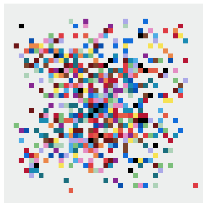
# Try the plot again
kelly_colors_III <-
ggplot(df, aes(x = x, y = y, fill = color)) +
geom_tile() + # Add tiles
scale_fill_identity() + # Use the colors stored as strings in the color column
theme_void() + # Remove axis labels and background
coord_equal() # Use equal aspect ratio
# Print the plot
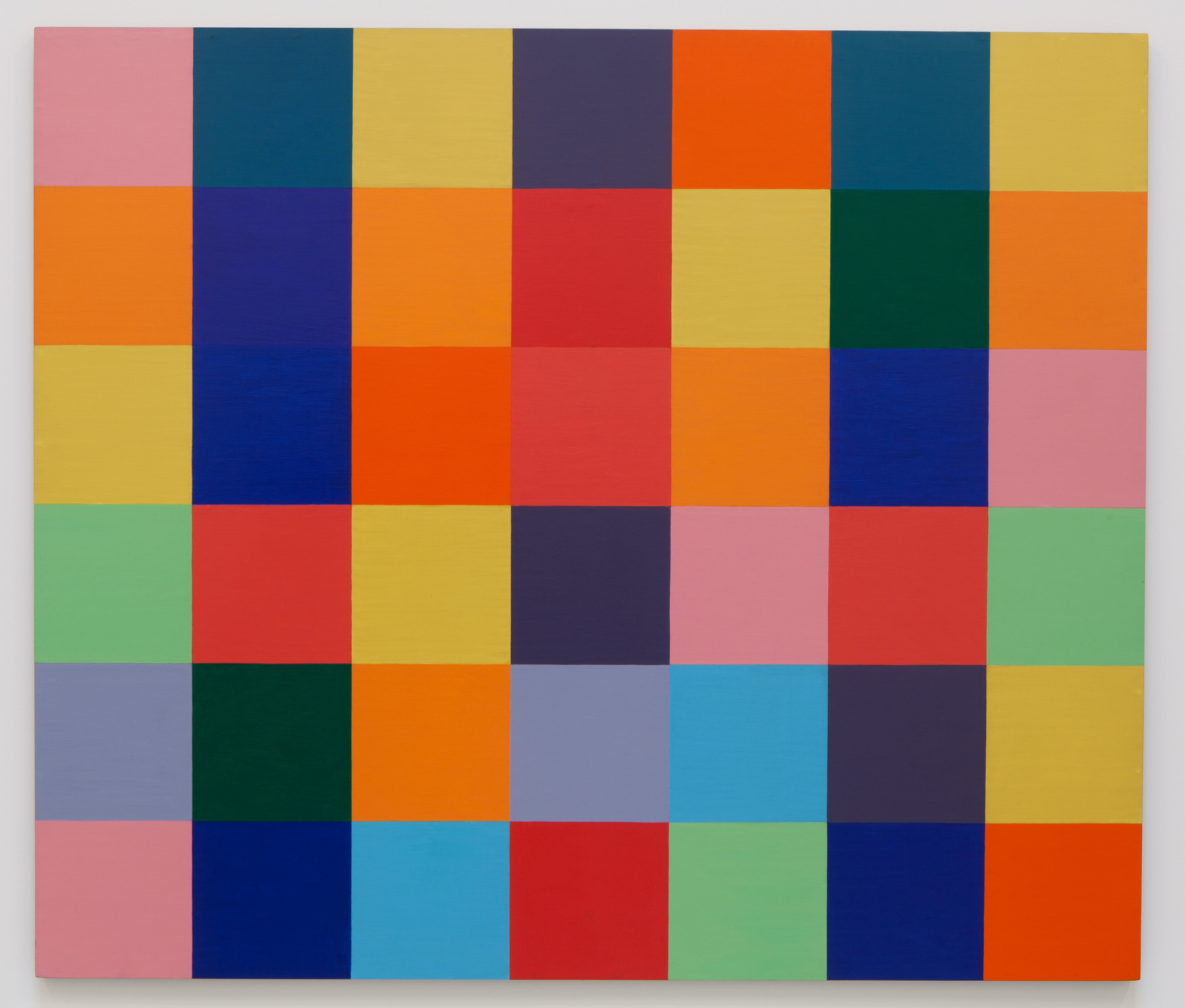
kelly_colors_III
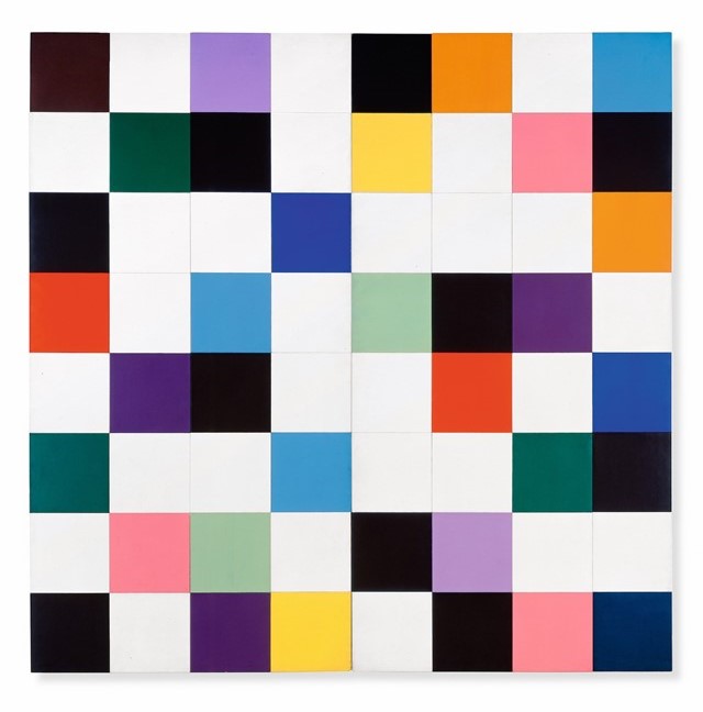
AYYYYYYYYY YAAAAAS!!! WHAT’S UP PARTY PEOPLLLLLE!!! This is some proGRESS! How exciting. Let’s look at it alongside piece III:
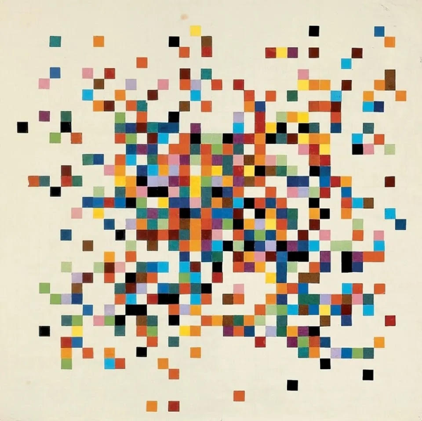
Now, I can finally see if the color probabilities really matter. A few days ago, I had discovered that some colors appeared more prominently than others, assuming my counting was correct. I actually considered inputting every single cell of his original into excel and running some actual calculations, but I gave myself a stern talking to and decided against that. For now.
The truth is, I don’t think I have enough information (from Kelly’s interviews or the piece itself) to know whether or not he actually intended there to be a higher instance of certain colors (namely black, blues, and oranges). While I do think that I could increase the probability of black, blues, oranges, etc, I know that would be VERY annoying to code unless I also asked the user to input the likelihood ratings for each of their chosen colors. Sounds like a larger cognitive lift than I’d like for both the user and myself 🥲
What I do know is that in Kelly’s pieces, no more than one or two squares of the same color ever seem to appear together, varying by piece, and I don’t even know how I’d set that constraint on my piece at this point. I think I’d have to take the color vector, make it into a matrix, then run through cell by cell and ask if the cells around it were the same color as it. If so, change the color to something other than its color or the colors of the cells around it. Or, assign the color vector to an empty matrix cell-by-cell in columns, checking each time to see that the color in the cells above and to the left don’t match. And I’d have to set conditions for edge cases (if col == 1, don’t check the cell to the left, if row == 1, don’t check the cell above, etc). And that sounds like a lot of work. Kelly was doing this by hand, essentially drawing colors from a hat. If he selected a color that was a duplicate of one of the colors he had already placed, he could simply toss it back in the hat and grab another random color. Watch, I’m gonna come back tomorrow and say I’ve decided to add this.
BUT! Kelly has several squares of the same color paired in piece 3! Just no more than two at a time. So.. I’d need to check to see if both adjacent squares were the same color, and only THEN take action to change the current square. See, now my brain wants to do this. It’s a curse.
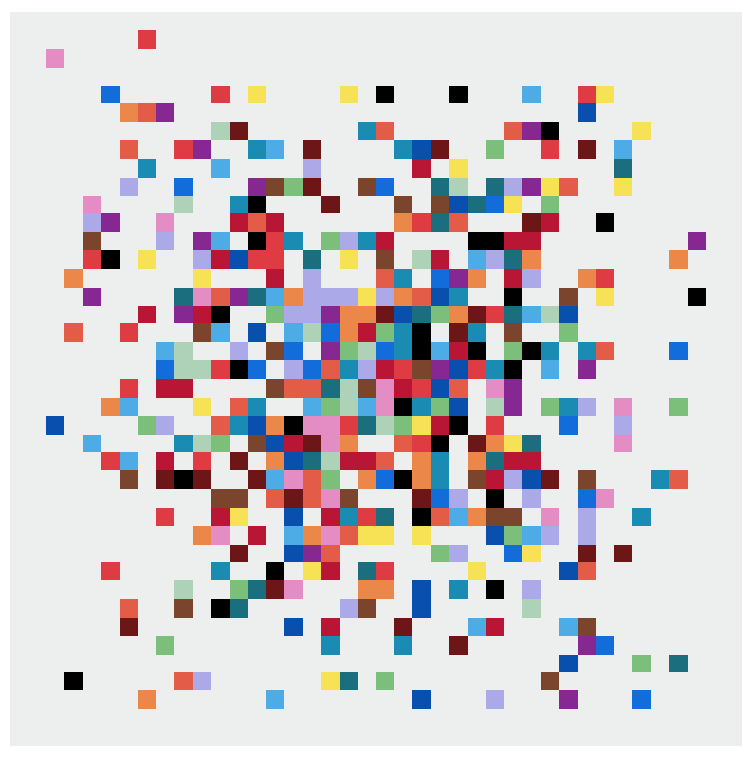
Ok, enough analysis. Let’s generate a few more and see what they look like! Then, it’s bedtime for this brain. I have a Brandon Sanderson novel to get back to and cats to feed.
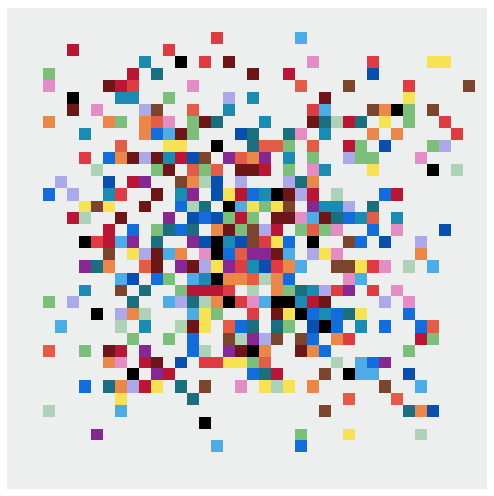
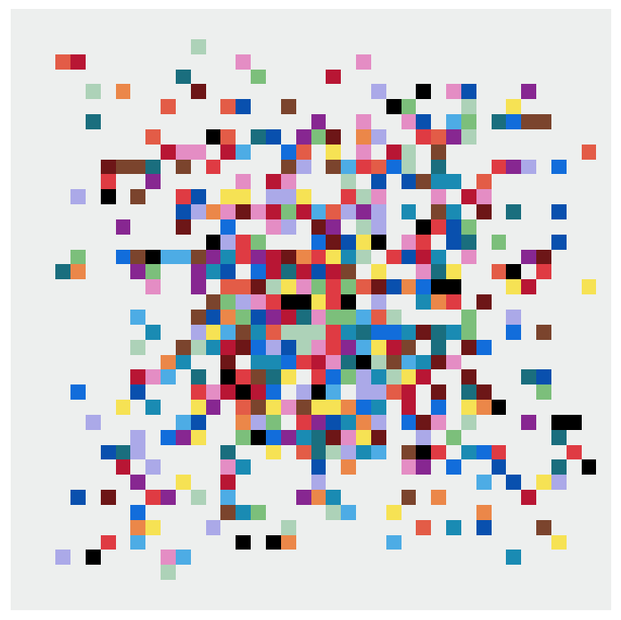

Words cannot express how happy these little color bombs make me. BEDTIME!
[Note from Future Libby: Past Libby really was exhausted but elated, and I love that for us. I remember these little coding mysteries running nonstop in my brain at that time.]
This was a lot of color and a lot of code. If you’re up for more (yes, there’s more), you can head to the sixth part in this series, and here’s the app in its current form if you’d like to play with it!.