size <- 40

circuits <- ifelse(size %% 2 == 0, size / 2, (size + 1) / 2)

# Analyze the probabilities found in piece III

# Create table of data from the piece
probs_table <-
  dplyr::tibble(
    circuit = 1:circuits,
    num_colored_in = c(0, 2, 4, 12, 19, 25, 30, 33, 37, 39,
                       39, 40, 39, 37, 34, 30, 25, 19, 12, 4),
    num_total = seq(from = 156, to = 4, by = -8)
)

# Calculate probabilities
probs_table <-
  probs_table |>
  mutate(prob_of_color = num_colored_in / num_total)

# Examine probability over circuits (outside in)
plot(probs_table$circuit, probs_table$prob_of_color)The Ellsworth Project: Part 2
R
Shiny
Documenting the creation of The Ellsworth App, in which I model probabilities and spin my wheels a lot, but have fun doing it.
February 20th, 2024
This was day two of development and I focused most of my time on modeling the probabilities found in Kelly’s Spectrum Colors Arranged by Chance III. I recreated some of my code from the previous day, including defining the size and number of circuits needed, and then I created a table of circuits and probabilities from my analysis (and by analysis I mean my physical counting that I hopefully did mostly correctly).
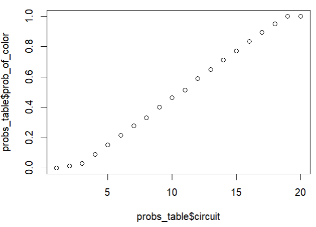
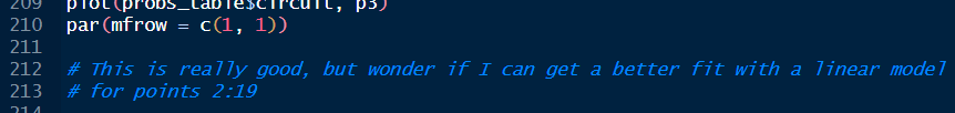
I noted that it was pretty dang linear with a slight sigmoid curve shape. It’s hilarious to me that I can see in my code where I took a note (in blue below) proposing an easy way out, which I briefly tested and then ignored because I wanted to test ALL THE THINGS. Spoiler: in the end, that initial idea was the way to go. Sort of.
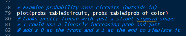
Below, I am simulating the sigmoid shape using my proposed method of just building the probability vector by assigning the first probability manually as 0, creating a linear growth of probabilities from 0 to 1, and then adding 1.0 manually as the last probability. Feel free to be baffled at my use of par(mfrow) here. I am a base coder at heart, and that’s what I instinctively use when I’m in a flow state and no one else needs to see what I’m making.
size <- 40

circuits <- ifelse(size %% 2 == 0, size / 2, (size + 1) / 2)

# Try simulating

sim_prob <- c(0, seq(0, 1, length.out = (circuits) - 2), 1)

# Examine actual probability over circuits (outside in)
# vs my simulated probabilities
par(mfrow = c(1, 2))
plot(probs_table$circuit, probs_table$prob_of_color)
plot(probs_table$circuit, sim_prob)
par(mfrow = c(1, 1))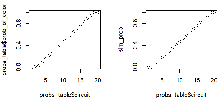
I thought this looked ok, but I knew it wouldn’t work scaled up to way larger sizes of grids. I wanted to see if I could approximate the shape using a sigmoid function. I relied on this web page about fitting a sigmoid curve in R to help me understand what I was doing, but I was not really fully in the know.
# x1 <- 1:(circuits - 1)
upper_asymp <- 1 # upper asymptote

# growth rate is (1/(length(probs_table$circuits)-2) if I'm going to
# add a 1 at the end
growth_rate <- round(1 / (circuits - 2), 3)

# time of maximum growth: x value at inflection
# (length(probs_table$circuits)/2 - 1)
x_at_inflection <- (circuits / 2) - 1

fitmodel1 <-
  nls(probs_table$prob_of_color[1:circuits - 1] ~ a / (1 + exp(-b * (x1 - c))),
      start = list(a = upper_asymp,
                   b = growth_rate,
                   c = x_at_inflection))

params <- coef(fitmodel1)

# This didn't work :(
# Error in nls(probs_table$prob_of_color[1:circuits - 1] ~ a/(1 + exp(-b *  :
#   parameters without starting value in 'data': prob_of_color, x1
After some googling, I figured out what that error was… probably… but my code still didn’t work. I abandoned the custom-named parameters and just defined a, b, and c in my starting code (using a best guess at what those might be). Hey, a new and different error! That’s called PROGRESS.
f_nls <- data.frame(x = 1:(circuits - 1),
                 y = probs_table$prob_of_color[1:circuits - 1])

upper_asymp <- 1 # upper asymptote
growth_rate <- round(1 / (circuits - 2), 3) # growth rate (1/(length(probs_table$circuits)-2) if I'm going to add a 1 at the end
x_at_inflection <- (circuits / 2) - 1 # time of maximum growth (x value at inflection, length(probs_table$circuits)/2 - 1)

fitmodel2 <- nls(y ~ I(a / (1 + exp(-b * (x - c)))),
                 data = df_nls,
                 start=list(a = 1,
                            b = 0.01351351,
                            c = 9))

# UGH WHY
# Error in nls(y ~ I(a/(1 + exp(-b * (x - c)))), data = df_nls, start = list(a = 1,  :
#   singular gradient
As it turns out, there’s a warning in the nls() documentation about a zero-residual problem when trying to converge. Ok! Someone on a stackoverflow post (that I can’t find) added a jitter to their data to correct for this, and that’s what I decided to do, as well as changing my start values up several times until it ran.
# Once more with JITTER
df_nls <- data.frame(x = 1:(circuits - 1),
                     y = jitter(probs_table$prob_of_color[1:circuits - 1]),
                     factor = 1)

fitmodel2 <- nls(y ~ I(a / (1 + exp(-b * (x - c)))),
                 data = df_nls,
                 start=list(a = 1.1,
                            b = 0.280,
                            c = 10))

params <- coef(fitmodel2)

# Inspect the estimates
estimated_points <-
  params[1] / (1 + exp(-params[2] * (probs_table$circuit[1:circuits - 1] - params[3])))

# code from blog post:
sigmoid = function(params, x) {
  params[1] / (1 + exp(-params[2] * (x - params[3])))
}

# Plot to see if the sigmoid curve is a good fit for my points
y2 <- sigmoid(params,1:19)
y <- probs_table$prob_of_color[1:circuits - 1]
plot(y2,type = "l")
points(y)
This curve was not a great fit for my points specifically, but an ok fit generally. I’m not super worried about overfitting an art piece, though, I’m just having fun, so I played around a bunch more to see if I could get a closer approximation. This was the closest I got by modifying the params.
params[1] <- 1.10
params[2] <- 0.280
params[3] <- 10.5

# Try plotting again
y2 <- c(NA, sigmoid(params, 1:circuits), NA)
y <- probs_table$prob_of_color
plot(y2, type = "l")
points(y)
I then thought, “You know what would be fun? SPLINES.” Why did I think this? Splines were my least favorite subject in undergrad. But I did it anyway because I love pain. The logspline package actually did pretty well and I didn’t die, but I also didn’t find a solution I loved, mostly because I couldn’t get the “early” probabilities (the ones occurring in the outermost circuits) to increase fast enough early enough. The probabilities increase more quickly in the first few circuits than they do in subsequent circuits. Don’t ask me why I used logspline estimation for data that was not log scale - I was not in a ‘thinking’ headspace, I was in a ‘throw-stuff-at-the-wall-and-see-what-sticks’ headspace.
library(logspline)

logspline(x = probs_table$prob_of_color,
          lbound = 0,
          ubound = 1,
          maxknots = 3)

fit <- logspline(x = probs_table$prob_of_color,
                 lbound = 0,
                 ubound = 1,
                 maxknots = 3)

probs1 <- qlogspline(p = probs_table$prob_of_color, fit = fit)

y <- probs_table$prob_of_color

plot(probs1,type = "l")
points(y)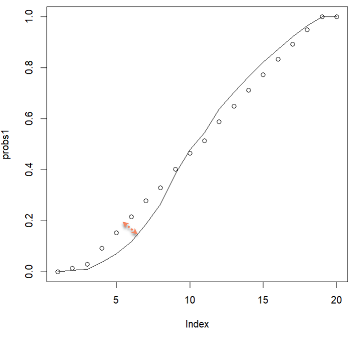
I decided that looking at only the probabilities wasn’t as helpful as how many colored-in-cubes they actually translated into at the scale of 40 by 40 and beyond. In that light, I decided to compare the number of squares filled with color in piece III to the number of squares filled in when using the probabilities from a couple of spline models.
logspline(x = probs_table$prob_of_color,
          lbound = 0,
          ubound = 1,
          maxknots = 3)

fit <- logspline(x = probs_table$prob_of_color,
                 lbound = 0,
                 ubound = 1,
                 maxknots = 3)

fit2 <- logspline(x = probs_table$prob_of_color,
                  lbound = -0.00000001,
                  ubound = 1,
                  knots = c(0.09090909, 0.46428571, 0.51315789))

probs1 <- qlogspline(p = probs_table$prob_of_color, fit = fit)
probs2 <- plogspline(q = probs_table$prob_of_color, fit = fit)
probs3 <- qlogspline(p = probs_table$prob_of_color, fit = fit2)

kellys <- probs_table$num_colored_in
p1 <- round(probs1 * probs_table$num_total)
p2 <- round(probs2 * probs_table$num_total)
p3 <- round(probs3 * probs_table$num_total)

par(mfrow = c(1, 3))
plot(probs_table$circuit, kellys)
plot(probs_table$circuit, p1)
plot(probs_table$circuit, p3)
par(mfrow = c(1, 1))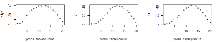
The three plots above show: left, the number of colored-in squares in Kelly’s piece III; center, the number of colored-in squares produced by my spline model 1 where I only supplied the max number of knots; right, the number of colored-in squares produced by my spline model 2 where I told it where to place the knots.
This is when I acknowledged that the logsplines work fine, but I still wasn’t getting the fit I wanted in the “early” circuits, and I didn’t want to mess with other polynomial spline equations to see if I could get a better fit, so… back to that initial gut instinct to create the probabilities linearly.
I wanted to isolate the middle 18 probabilities. I knew the first probability should always be 0 and the last should always be 1, so I wanted to see what the middle 18 looked like when simulated linearly compared to the actual piece.
# Fit a linear model on the inner 18 probs
fitlm <-
  lm(probs_table$prob_of_color[3:circuits - 1] ~ probs_table$circuit[3:circuits - 1])

# list of numbers 2 through 19
circuitlist <- list(probs_table$circuit[3:circuits - 1])

# create probs along the line of best fit
lm1_pred <- predict.lm(fitlm, circuitlist)

# Plot them compared to the original middle 18 probs
par(mfrow = c(1, 2))
plot(probs_table$circuit[3:circuits-1], probs_table$prob_of_color[3:circuits - 1])
plot(probs_table$circuit[3:circuits-1], lm1_pred)
par(mfrow = c(1, 1))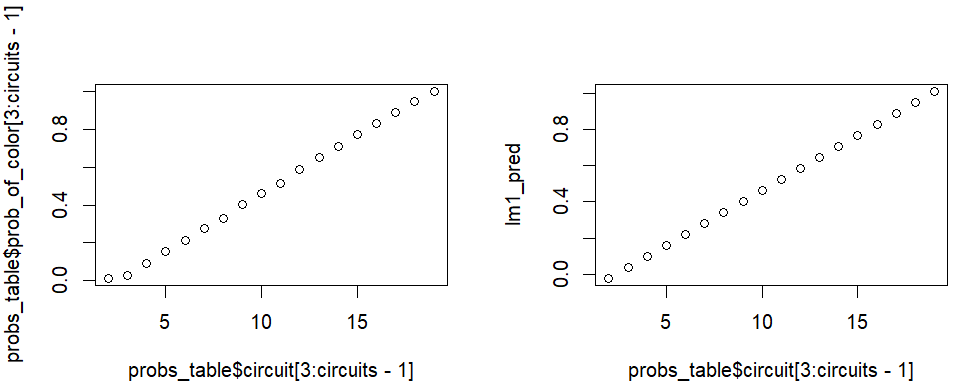
It works great for at least the 3rd value onwards, but for some reason I couldn’t let it go at that. I kept playing. I examined the probabilities again and looked at their diffs (the amount they increase with each circuit, basically, circuit 2’s probability minus circuit 1’s probability, then circuit 3’s minus circuit 2’s, and so on).
diff(probs_table$prob_of_color)

# > diff(probs_table$prob_of_color)
# [1] 0.01351351 0.01505792 0.06233766 0.06231672
# [5] 0.06229143 0.06226054 0.05222222 0.07217391
# [9] 0.06211180 0.04887218 0.07507740 0.06176471
# [13] 0.06153846 0.06118881 0.06060606 0.05952381
# [17] 0.05714286 0.05000000 0.00000000

# So, for the first 10% of the values (the first 2 of 20 here), the increase is
# about .014. Then, for the other 90% of values, the increase is about
mean(diff(probs_table$prob_of_color[3:20])) # 0.05714286
I found that the first 10% of values scaled by about .014 each time, and then the rest of the circuits increased by about .057 each circuit, on average.
After some flailing, I wrote a function that would naively calculate how many probabilities to create in the first 10% of the number of circuits, and then the other 90%. At this point, I was totally ignoring the fact that I could just calculate the first 10% and then do simple subtraction (total number of circuits minus the number of circuits I decided was 10%) to find the last 90%.
get_prob_vector <- function(circuits){

  first10perc <- seq(0, 0.02857143, length.out = round(circuits * 0.10) + 1)
  last90perc <- seq(0.02857143, 1, length.out = round(circuits * 0.90) - 1)[-1]

  prob_vector <- c(first10perc, last90perc, 1)

  return(prob_vector)
}
Watch me flail some more:
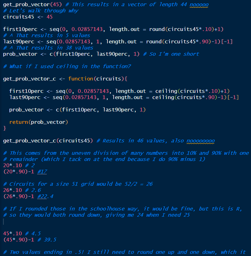
This goes on for some time, so I’ll spare you. Eventually, I got to a solution I liked (STILL IGNORING THE FACT THAT I COULD JUST SUBTRACT), and that passed tests, but that didn’t give me the results I wanted because, well… it wasn’t gonna scale up or down without also calculating a different set of probabilities for the last 10% of the circuits (the ones on the inside/center). Basically, the upper-right part of the sigmoid shape wasn’t going to get larger as the grid size increased, and I didn’t like that. As the size of any given grid increased, the density of color at the center would decrease in proportion to the rest of the piece.
get_prob_vector_r <- function(circuits){

  first10perc <- seq(0, 0.02857143, length.out = round(circuits * 0.10) + 1)
  last90perc <- seq(0.02857143, 1, length.out = round((circuits * 0.90) - 1))[-1]

  prob_vector <- c(first10perc, last90perc, 1)

  return(prob_vector)
}

# Test it at smaller sizes
circuits45 <- 45
get_prob_vector_r(circuits45) # Gives me 45, good

prob_vectors_test <- map(1:65, get_prob_vector_r)

prob_vector_lengths <- map(prob_vectors_test, length)

identical(unlist(prob_vector_lengths[-1]), 2:65) #TRUE!

# Ok, that worked for circuits of 1 to 65!

# What about huge sizes?

prob_vectors_test <- map(66:200, get_prob_vector_r)

prob_vector_lengths <- map(prob_vectors_test, length)

identical(unlist(prob_vector_lengths), 66:200) # OMG ALSO TRUE

# Can I plot the shape of the probabilities on Kelly's vs my 40 vs other?
par(mfrow = c(1, 3))
plot(probs_table$circuit, probs_table$prob_of_color, pch = 16)
plot(probs_table$circuit, get_prob_vector_r(circuits), pch = 16)
plot(1:65, get_prob_vector_r(65), pch = 16)
# at a size of 65, the top curve is too small
par(mfrow = c(1, 1))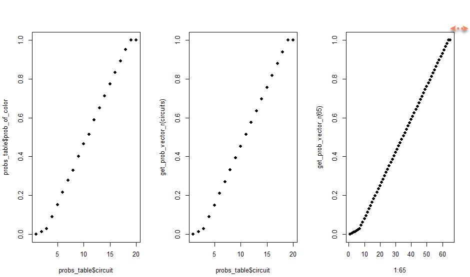
See? Up there at the top right. On the left is the art piece’s probabilities. Center is my created probabilities using my function on a size 40 x 40 grid. On the right is my function used to create a larger 65 x 65 sized grid, showing that the tail end of the shape is too small. I need the last 10% of the probabilities to all be 1.
Here’s some more flailing:
get_prob_vector_80 <- function(circuits){

  first10perc <- seq(0, 0.02857143, length.out = round(circuits * 0.10) + 1)
  middle80perc <- seq(0.02857143, 1, length.out = round((circuits * 0.80)))[-1]
  last10perc <- rep(1, round(circuits * 0.10))

  prob_vector <- c(first10perc, middle80perc, last10perc)

  return(prob_vector)
}

get_prob_vector_80(45) # gives me 44, noooo

# This works with circuits == 20
first10perc <- seq(0, 0.02857143, length.out = round(circuits * 0.10) + 1) # 3 values
middle80perc <- seq(0.02857143, 1, length.out = round((circuits * 0.80)))[-1] #15
last10perc <- rep(1, round(circuits * 0.10)) # 2

# But with circuits == 45
first10perc <- seq(0, 0.02857143, length.out = round(45 * 0.10) + 1) # 5 (4.5 rounded to 4 +1)
middle80perc <- seq(0.02857143, 1, length.out = round((45 * 0.80)))[-1] # 35 (36-1, this is ok)
last10perc <- rep(1, round(45 * 0.10)) # 4 (4.5 rounded to 4 but needs to be 5)

# What if I added the +1 into the round in first10perc?
get_prob_vector_80_r <- function(circuits){

  first10perc <- seq(0, 0.02857143, length.out = round((circuits * 0.10) + 1))
  middle80perc <- seq(0.02857143, 1, length.out = round((circuits * 0.80)))[-1]
  last10perc <- rep(1, round(circuits * 0.10))

  prob_vector <- c(first10perc, middle80perc, last10perc)

  return(prob_vector)
}

get_prob_vector_80_r(45) # gives me 45, good

# Run test on 2:200
prob_vectors_test2 <- map(2:200, get_prob_vector_80_r)

prob_vector_lengths2 <- map(prob_vectors_test2, length)

identical(unlist(prob_vector_lengths2), 2:200) # FALSE BOO

# Ok, well, I know I can get 10% and 90% to work and that it's a pretty
# good approximation of Kelly's algorithm. Maybe I leave it at that.

# If I can get the length.out to work for 90%, then can I just take away
# a percentage of that? What percentage of 90% of a whole is 10% of that whole?
# For 100, that would be 10 out of 90 which is .11111repeating
# and that won't always be a round number
That is painful to look at. Now we get to the point where I figure out how to simplify this process. I’m so close to understanding basic math here.
get_prob_vector_r_prop <- function(circuits){

  first10perc <- seq(0, 0.02857143, length.out = round(circuits * 0.10) + 1)

  last90perc_length <- round((circuits * 0.90) - 1)

  last10perc_length <- circuits - length(first10perc)

  middle80perc_length <- last90perc_length - last10perc_length

  middle80perc <- seq(0.02857143, 1,
                      length.out = middle80perc_length + 2)[-c(1, middle80perc_length + 2)]

  last10perc <- rep(1, last10perc_length)

  prob_vector <- c(first10perc, middle80perc, last10perc)

  return(prob_vector)
}

# Did that work?

# Run test on 2:200
prob_vectors_test3 <- map(2:200, get_prob_vector_r_prop)

prob_vector_lengths3 <- map(prob_vectors_test3, length)

identical(unlist(prob_vector_lengths3), 2:200) # TRUE OMG I DIE
I was so stoked! Look at that last code comment 😂 I then plotted my last plot again comparing Kelly’s probabilities to my simulated probabilities at size 40 x 40, and then 65 x 65. BAM! The tail end of the sigmoid curve now scales proportionally to the rest of the piece!
par(mfrow = c(1, 3))
plot(probs_table$circuit, probs_table$prob_of_color, pch = 16)
plot(probs_table$circuit, get_prob_vector_r_prop(circuits), pch = 16)
plot(1:65, get_prob_vector_r_prop(65), pch = 16)
par(mfrow = c(1, 1))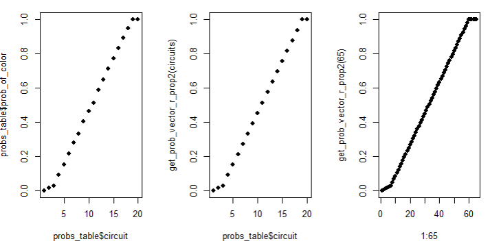
Can we stop and appreciate that I’m not solving world hunger? I’m recreating an art piece from 1951. I know it’s not super important work, but I was having soooo much fun.
At this point, I needed to shift to actually assigning probabilities to a matrix. I knew I could do this in one of two ways:
- I could build a quadrant of probabilities and mirror it as mentioned way up above
- Or, I could build the matrix in a spiral, like in this video about spiral matrices (which I enjoyed and which really got me in the right headspace for doing the quadrant method!)
I remember trying to go to sleep at this point after watching that YouTube video, but it was hopeless, my ADHD brain was hyper-focused. I needed to get a few more things down on (digital) paper before my brain would let go and let me sleep.
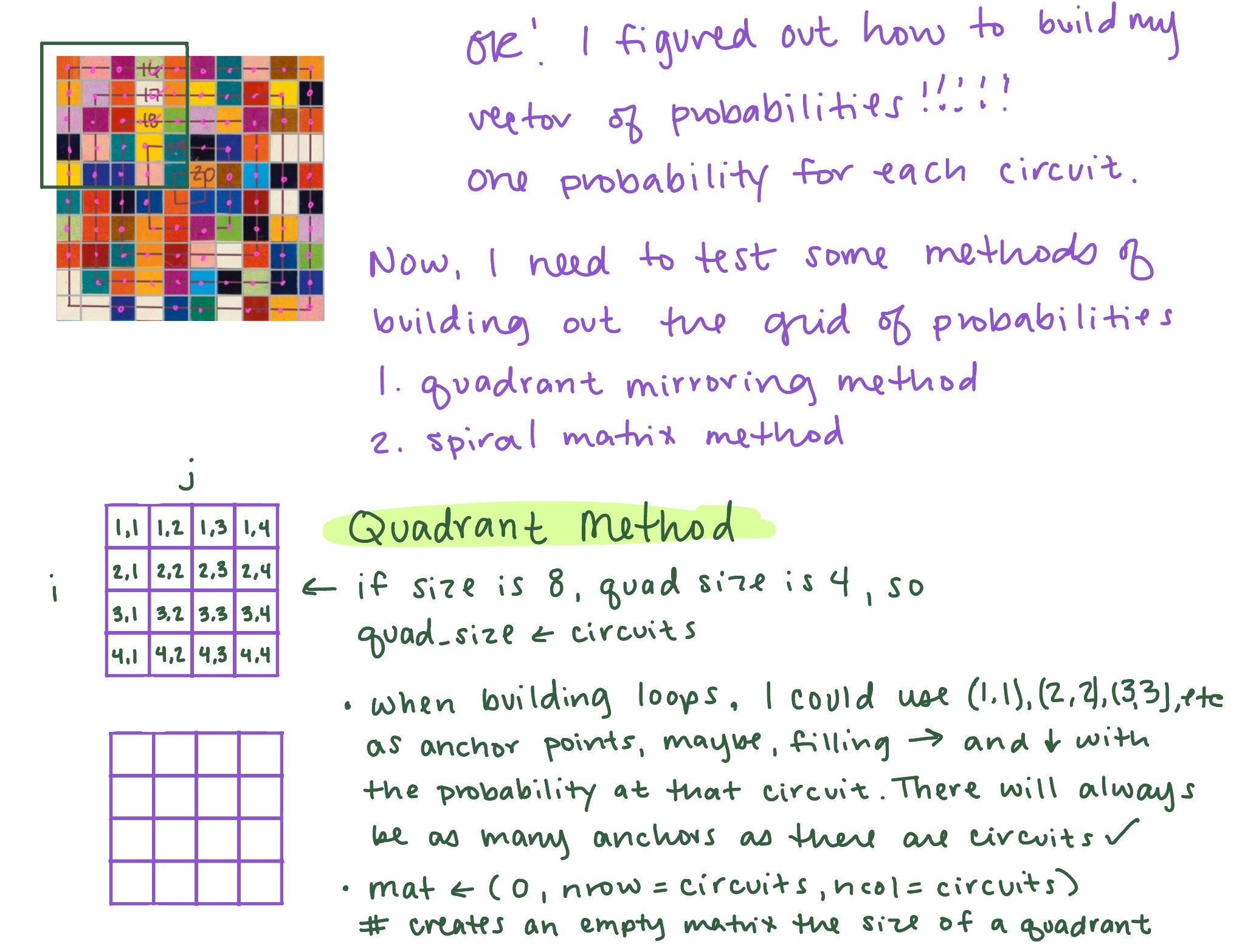
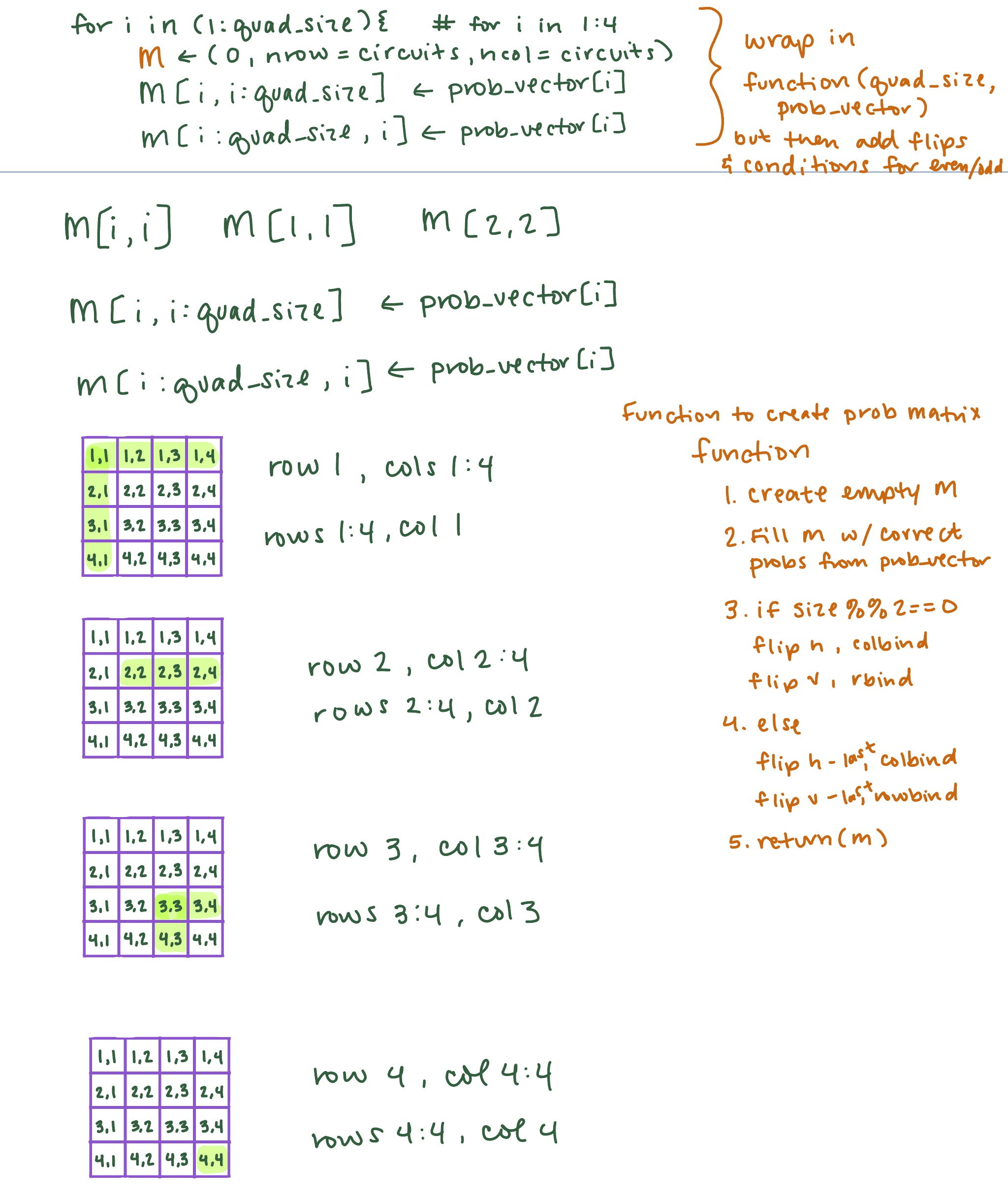
And then I went to bed hoping that my handwritten code would actually work 🥱
You can find the third post in the series here, and here’s the app in its current form if you’d like to play with it!.